We're sunsetting PodQuest on 2025-07-28. Thank you for your support!

cover of episode “Compressed Computation is (probably) not Computation in Superposition” by Jai Bhagat, Sara Molas Medina, Giorgi Giglemiani, StefanHex

“Compressed Computation is (probably) not Computation in Superposition” by Jai Bhagat, Sara Molas Medina, Giorgi Giglemiani, StefanHex

2025/6/23

Shownotes Transcript

Audio note: this article contains 113 uses of latex notation, so the narration may be difficult to follow. There's a link to the original text in the episode description.

This research was completed during the Mentorship for Alignment Research Students (MARS 2.0) Supervised Program for Alignment Research (SPAR spring 2025) programs. The team was supervised by Stefan (Apollo Research). Jai and Sara were the primary contributors, Stefan contributed ideas, ran final experiments and helped writing the post. Giorgi contributed in the early phases of the project. All results can be replicated using this codebase. Summary

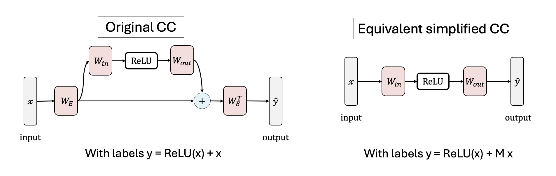
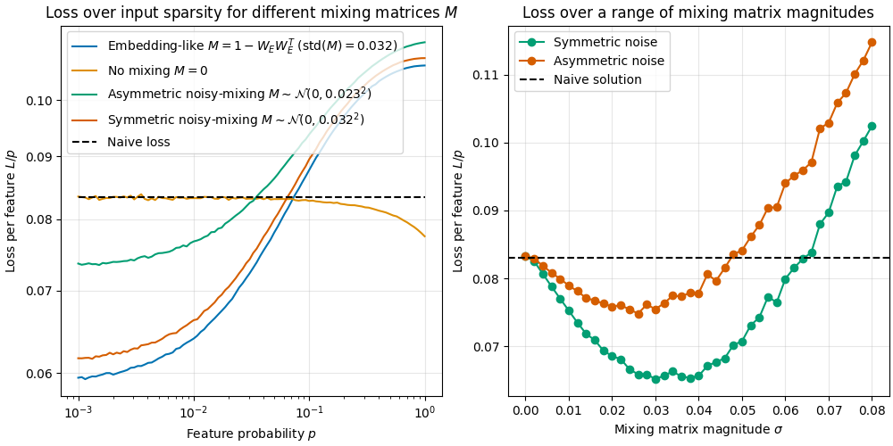
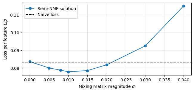
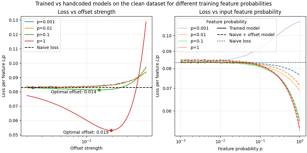
We investigate the toy model of Compressed Computation (CC), introduced by Braun et al. (2025), which is a model that seemingly computes more non-linear functions (100 target ReLU functions) than it has ReLU neurons (50). Our results cast doubt on whether the mechanism behind this toy model is indeed computing more functions [...]

Outline:

(00:59) Summary

(02:42) Introduction

(04:38) Methods

(06:34) Results

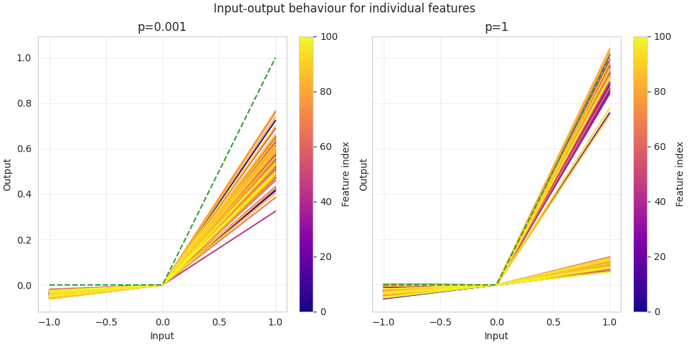
(06:37) Qualitatively different solutions in sparse vs. dense input regimes

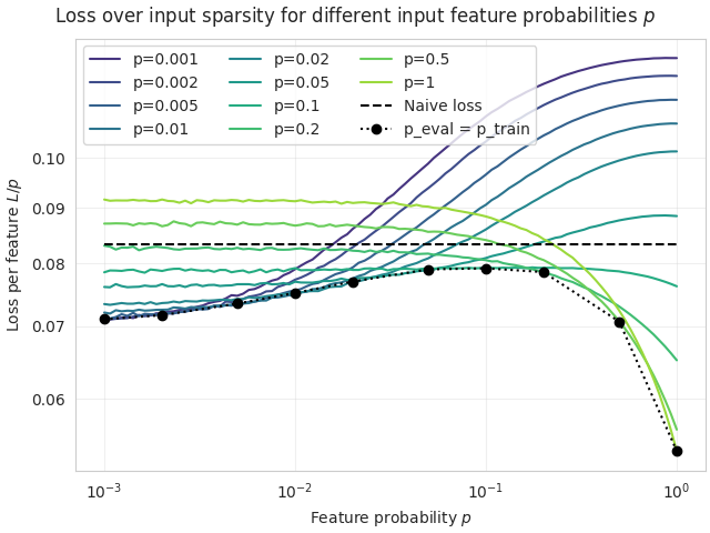
(09:49) Quantitative analysis of the Compressed Computation model

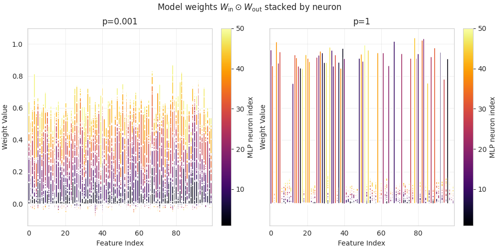
(13:09) Mechanism of the Compressed Computation model

(18:11) Mechanism of the dense solution

(20:55) Discussion

The original text contained 9 footnotes which were omitted from this narration.

First published: June 23rd, 2025

Source: https://www.lesswrong.com/posts/ZxFchCFJFcgysYsT9/compressed-computation-is-probably-not-computation-in)

Narrated by TYPE III AUDIO).

Images from the article: Figure 1: The original model architecture from Braun et al. (2025), and our simpler equivalent model. ))) $Figure 4: Weights representing each input feature, split by neuron. Each bar corresponds to a feature (x-axis) and shows the adjusted weight value from __T3A_INLINE_LATEX_PLACEHOLDER___W_{\text{out}} \odot W_{\text{in}}___T3A_INLINE_LATEX_END_PLACEHOLDER__, split by neuron index (color). The CC solution (left) combinations of neurons to represent each feature (to around 70%), whereas the dense solution (right) allocates a single neuron to fully (~100%) represent 50 out of 100 features.$ ) $Figure 5, left: Loss per feature as a function of input sparsity, for different choices of __T3A_INLINE_LATEX_PLACEHOLDER___M___T3A_INLINE_LATEX_END_PLACEHOLDER__. We compare an embedding-like __T3A_INLINE_LATEX_PLACEHOLDER___M___T3A_INLINE_LATEX_END_PLACEHOLDER__ (Braun et al. 2025, blue) to a fully random __T3A_INLINE_LATEX_PLACEHOLDER___M___T3A_INLINE_LATEX_END_PLACEHOLDER__ (green) and a symmetric __T3A_INLINE_LATEX_PLACEHOLDER___M___T3A_INLINE_LATEX_END_PLACEHOLDER__ (red) which is a random lower diagonal matrix mirrored; in both cases we set the magnitude if __T3A_INLINE_LATEX_PLACEHOLDER___M___T3A_INLINE_LATEX_END_PLACEHOLDER__ that leads to the lowest loss. For comparison we also show a model trained on __T3A_INLINE_LATEX_PLACEHOLDER___M=0___T3A_INLINE_LATEX_END_PLACEHOLDER__ (yellow). We find that all non-zero __T3A_INLINE_LATEX_PLACEHOLDER___M___T3A_INLINE_LATEX_END_PLACEHOLDER__ lead to a qualitatively similar profile, and that a symmetrized random __T3A_INLINE_LATEX_PLACEHOLDER___M___T3A_INLINE_LATEX_END_PLACEHOLDER__ almost gives the same result as Braun et al. (2025).Right: Optimal loss as a function of mixing matrix magnitude __T3A_INLINE_LATEX_PLACEHOLDER___\sigma___T3A_INLINE_LATEX_END_PLACEHOLDER__ (separately trained for every __T3A_INLINE_LATEX_PLACEHOLDER___\sigma___T3A_INLINE_LATEX_END_PLACEHOLDER__). For small __T3A_INLINE_LATEX_PLACEHOLDER___\sigma___T3A_INLINE_LATEX_END_PLACEHOLDER__ the loss linearly decreases with the mixing matrix magnitude, suggesting the loss advantage over the naive solution stems from the mixing matrix __T3A_INLINE_LATEX_PLACEHOLDER___M___T3A_INLINE_LATEX_END_PLACEHOLDER__. At large values of __T3A_INLINE_LATEX_PLACEHOLDER___\sigma___T3A_INLINE_LATEX_END_PLACEHOLDER__, the loss increases again.$ ) $Figure 6: Training a model on the noisy dataset (__T3A_INLINE_LATEX_PLACEHOLDER___M \neq 0___T3A_INLINE_LATEX_END_PLACEHOLDER__), and then fine-tuning on the clean __T3A_INLINE_LATEX_PLACEHOLDER___M=0___T3A_INLINE_LATEX_END_PLACEHOLDER__ case. We see that the loss jumps back up as soon as we switch to the clean task. This is evidence against the hypothesis that the CC solution wasn't learned on the clean case just due to training dynamics.$ ) $Figure 7, left: Cosine similarity between various eigen- and singular vectors (x-axis) and MLP neuron directions (y-axis). We show eigenvectors in the top panels, singular vectors in the bottom panels, the __T3A_INLINE_LATEX_PLACEHOLDER___W_{\rm in}___T3A_INLINE_LATEX_END_PLACEHOLDER__ matrix in the left panels, and the __T3A_INLINE_LATEX_PLACEHOLDER___W_{\rm out}___T3A_INLINE_LATEX_END_PLACEHOLDER__ matrix in the right panels. In all cases we see that the top-50 vectors (sorted by eigen- / singular value) have significant dot product with the neurons, while the remaining 50 vectors have near-zero dot products (black).Right: We test how well the ReLU-free MLP (i.e. just the __T3A_INLINE_LATEX_PLACEHOLDER___W_{\rm out} W_{\rm in}___T3A_INLINE_LATEX_END_PLACEHOLDER__ projection) preserves various eigen- (orange) and singular (blue) directions. Confirming the previous result, we find the cosine similarity between the vectors before and after the projection to be high for only the top 50 vectors.$ ) $Figure 8, left: Scatter plot of the entries of the product __T3A_INLINE_LATEX_PLACEHOLDER___W_{\rm out} W_{\rm in}___T3A_INLINE_LATEX_END_PLACEHOLDER__ and the mixing matrix __T3A_INLINE_LATEX_PLACEHOLDER___M___T3A_INLINE_LATEX_END_PLACEHOLDER__; the entries are clearly correlated. The diagonal entries of __T3A_INLINE_LATEX_PLACEHOLDER___W_{\rm out} W_{\rm in}___T3A_INLINE_LATEX_END_PLACEHOLDER__ are offset by a constant, and seem to be correlated at a higher slope.Right: Visualization of the MLP weight matrices __T3A_INLINE_LATEX_PLACEHOLDER___W_{\rm in}___T3A_INLINE_LATEX_END_PLACEHOLDER__ and __T3A_INLINE_LATEX_PLACEHOLDER___W_{\rm out}___T3A_INLINE_LATEX_END_PLACEHOLDER__. We highlight that __T3A_INLINE_LATEX_PLACEHOLDER___W_{\rm in}___T3A_INLINE_LATEX_END_PLACEHOLDER__ is has mostly positive entries (this makes sense as it feeds into the ReLU), and both matrices have a small number of large entries.$ ) $Figure 9: Loss of the SNMF solution, compared to the naive solution. Like in Figure 5b, the solution does better than the naive loss for a range of __T3A_INLINE_LATEX_PLACEHOLDER___\sigma___T3A_INLINE_LATEX_END_PLACEHOLDER__ values though the range is smaller and the loss is higher than for the trained model.$ ) $Figure 10, left: A non-zero offset in the __T3A_INLINE_LATEX_PLACEHOLDER___W_{\rm out}___T3A_INLINE_LATEX_END_PLACEHOLDER__ entries of unrepresented features improves the loss in the dense regime. We determine the optimal value empirically for each input feature probability __T3A_INLINE_LATEX_PLACEHOLDER___p___T3A_INLINE_LATEX_END_PLACEHOLDER__.Right: This hand-coded naive + offset model (dashed lines) consistently matches or outperforms the model trained on clean labels (solid lines) in the dense regime. (Note that this plot only shows the clean dataset (__T3A_INLINE_LATEX_PLACEHOLDER___M=0___T3A_INLINE_LATEX_END_PLACEHOLDER__) which is why no solution outperforms the naive loss in the sparse regime.)$ ) Apple Podcasts and Spotify do not show images in the episode description. Try Pocket Casts), or another podcast app.